Experimental considerations

There are several important factors to a successful repeat instability experiment and things to consider when using this package.

Unique sample IDs

(required)

Each sample has a unique id, usually the file name. If there are duplicate file names they will be appended with a number. This is important because if you use any of the metadata options, those file names will no longer match up.

Index assignment and metrics

(optional)

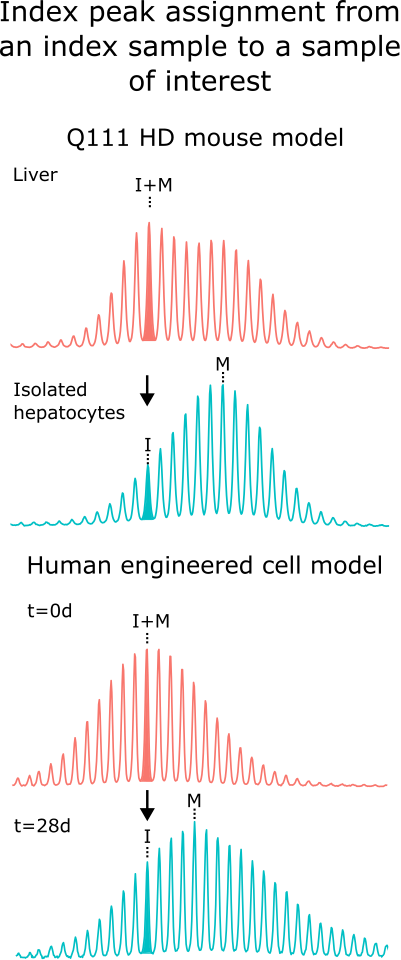
In many experiments, the inherited or starting repeat length (referred to here as the index peak) is a critical reference point for downstream metrics. By default, the index peak corresponds to the modal peak of the chosen index sample. In a second sample of interest, the equivalent index peak is identified as the peak closest in repeat size to the index sample’s modal peak. In the simplest scenario, the modal peak remains the same in both samples, so the index peak is also the modal in each. In other cases, however, the modal peak of the sample of interest may have shifted due to repeat expansion or contraction; in these situations, this software can assign the index peak based on its correspondence to the modal peak of the index sample.

This allows, for example, an expanded repeat knock-in mouse liver sample to define the inherited repeat length used to assess expansion in the isolated hepatocytes, or a time-zero sample to define the starting repeat length for a cell line monitored over time (Figure 1).

This is indicated with a TRUE in the metrics_baseline_control column of the metadata. Samples are then grouped together with the metrics_group_id column of the metadata. Multiple samples can be metrics_baseline_control, which can be helpful for the average repeat change metric to have a more accurate representation of the average repeat at the start of the experiment.

Index peak assignment and benchmarking of instability metrics. (A) Example of index peak assignment in mouse tissues (top) and cell lines (bottom). In the mouse liver sample (red), the index (I) peak corresponds to the modal (M) peak, reflecting the inherited repeat length. This index peak is then applied to the isolated hepatocyte sample (blue), where somatic expansion shifts the modal peak toward larger repeat sizes. In the cell line experiment (bottom), the modal peak of the time-zero sample (red) is used as the index peak for the 28-day sample (blue).

Fragment analysis batch effects

(optional)

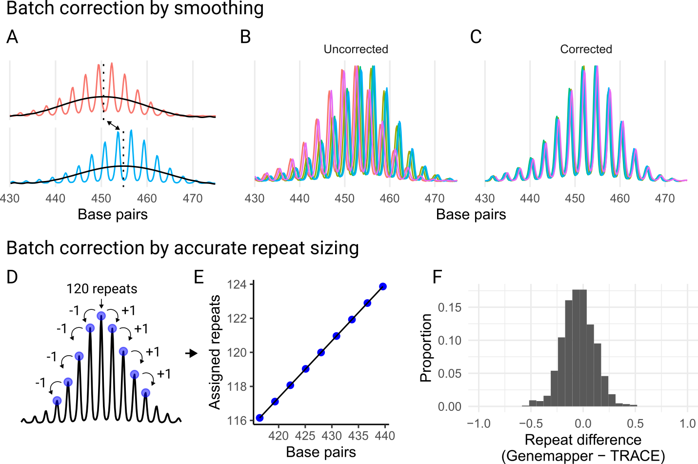
A challenge in fragment analysis is that repeat-containing amplicons do not migrate linearly with the ladder fragments. The spacing, in base pairs, between consecutive amplicon peaks is often smaller than the full repeat. This results in an underestimation of repeat length if you just convert from base-pair size. These differences are not always consistent across runs which can result in batch effects in the repeat size. So, if the repeat length is to be directly compared for samples from different runs, this batch effect needs to be corrected. We provide two approaches, either simple correction ‘batch’ through trace smoothing and comparison (Figure 2 A-C), or accurate repeat sizing ‘repeat’ (Figure 2 D-F).

This is only relevant when the absolute size of a amplicons are compared for grouping metrics as described above (otherwise instability metrics are all relative and it doesn’t matter that there’s systematic batch effects across runs), when plotting traces from different runs, or if an accurate repeat length is desired.

There are two main correction approaches that are somewhat related: either ‘batch’ or ‘repeat’ in call_repeats(). Batch correction is relatively simple and just requires you to link samples across batches by indicating them from metadata. But even though the repeat size that is return will be precise, it will not be accurate and underestimates the real repeat length. By contrast, repeat correction can be used to accurately call repeat lengths (which also corrects the batch effects). However, the repeat correction will only be as good as your sample(s) used to call the repeat length, so this can a challenging and advanced feature. You need to use a sample that reliably returns the same peak as the modal peak, or you need to be willing to understand the shape of the distribution and manually validate the repeat length of each control sample for each run.

Correcting batch effects to standardize fragment analysis runs. (A) In the first approach, batch correction factors (red and blue indicate the same sample but different run) are determined by smoothing (black line) the trace and identifying maxima (vertical dotted lines), aligning traces even when they differ in their modal peaks. In this example, the top panel’s modal peak is one repeat unit smaller than that of the bottom panel when converted from base pairs. (B) The same sample from different runs is overlaid, with colors indicating different fragment analysis runs. (C) The same samples as in B, shown after applying the batch correction factor. (D) In the second approach, samples of known repeat lengths are used to assign the modal repeat length, and neighboring peaks are identified sequentially by jumping from peak to peak. (E) A linear model is created using the assigned repeats and their corresponding base pair sizes, which is then used to predict the modal repeat length of all samples within a run. (F) The difference between the modal repeat lengths called by GeneMapper and TRACE for 872 samples across 32 runs.

Ladders

If starting from fsa files, the GeneScan™ 1200 LIZ™ dye Size Standard ladder assignment may not work very well due to how the ladder assignment algorithm works. It is optimized for scenarios where all peaks of the ladder are resolved, which is usually the case for GeneScan™ 500 LIZ™ or GeneScan™ 600 LIZ™. To work in this package, Ladders like 1200 LIZ™ need to be run on the instrument in such a way that all of the peaks are resolved, otherwise they all blend together at the end. However, these ladders can be fixed by playing with the various parameters (or supplying a truncated version of the GeneScan™ 1200 LIZ™) or manually with the built-in fix_ladders_interactive() app.